Using Excel to Create Local Thresholds

You can use formulas in Excel to create local thresholds to use in DataLoader.

Creating the Input File

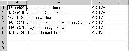
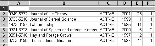
Create an Excel spreadsheet with the ISSNs in the first column (column A). You can use the journal names in column B to aid in identification (optional). The third column should contain the value ACTIVE (case-sensitive) if you also want to activate the portfolios for these journals during the same action (optional).

Use the next three columns to input the years, volumes, and issues of the journals.

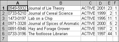
There are two methods for creating the input file.

Method 1

1. Leave blank columns to the left of each of these numerical values.

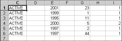
2. Enter the following value in the D1 cell (the first part of the local threshold):

$obj->parsedDate(“>=”,

3. Use the Fill feature in Excel to populate the column (use the fill handle at the right bottom side of each selected cell or use Edit > Fill Down).

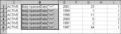
4. Do the same for cell F1, H1, and J1, inserting the values comma, comma, and end parenthesis.

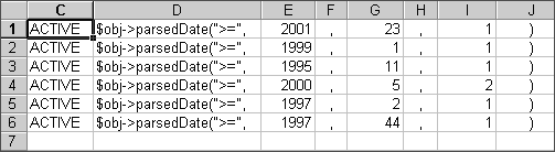
5. In the column to the right of the last one, insert the following formula:

=D1&E1&F1&G1&H1&I1&J1

6. Use the Fill feature in Excel to populate the column (use the fill handle at the right bottom side of each selected cell or use Edit > Fill Down).

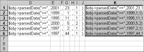
You now have a syntactically correct date threshold. To complete the process, make sure the cells in this column become text values instead of formulas.

7. Select the column with the threshold values (click the letter at the top). Press <ctrl> +c to paste the material into the buffer.
8. Select the next column (click the letter at the top—in our example, column L).
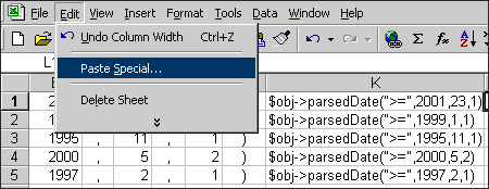
9. From the Edit menu, select Paste Special > Value.

10. Delete all the workspace columns containing information you no longer need.

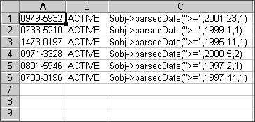
Moving extra data produces the following: columns A (ISSN), B (ACTIVE), and C (LOCAL THRESHOLD).

Method 2

1. Insert a blank row at the top of the Excel file.

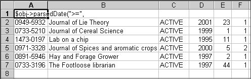
2. Insert the following value in the A1 cell:

$obj->parsedDate(“>=”,

3. Insert the following formula in G2 cell:

=$A$1&D2&”,”&E2&”,”&F2&”)”

4. Use the Fill feature in Excel to populate the column (use the fill handle at the right bottom side of each selected cell or use Edit > Fill Down).

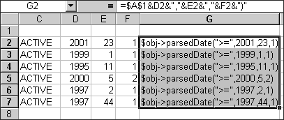
You now have a syntactically correct threshold. However, the cells in this column still consist of a formula only, not a text value.

5. Select the column with the threshold values (click the letter at the top). Press <ctrl> + c to paste the material into the buffer.
6. Select the next column over (click the letter at the top—in our example, column H.
7. From the Edit menu, select Paste Special > Values.

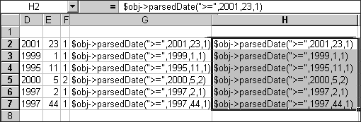
8. Delete all the workspace columns containing information you no longer need.
9. Remove extra data to produce the following: columns A (ISSN), B (ACTIVE), and C (LOCAL THRESHOLD).